Introduction

The idea behind quantum computers is that their computation capability is exponentially faster against classical hardware. A quantum algorithm running on quantum computer benefits from the so-called quantum properties: superposition, entanglement, and interference.

Superposition is the quantum phenomenon where a quantum system can exist in multiple states or places at the same time.

Entanglement is a strong correlation existing between two or more quantum particle.

Interference is a byproduct of superposition that allows to bias the measurement of a qubit toward a desired state or set of states.

The fact that Quantum Computing is faster than traditional computing can be demonstrated through Grover’s algorithm via Qiskit, an open-source framework for quantum development that provides tools for creating and manipulating quantum programs on IBM Quantum Experience (an online platform that allows public access to cloud-based IBM’s quantum computing services).

Demonstrating Grover’s algorithm with Qiskit

The second most famous quantum algorithm that demonstrates how a quantum computer outperforms a classical computer is Grover’s algorithm, which focuses on searching an element in an unordered list, quadratically faster than the best classical algorithm. You can find the complete example here, but let’s try to recap its main concepts.

Suppose you have a list of N unsorted items and you have to look for the position of an element. With a classical algorithm, you’d have to check N/2 elements on average to find the element you are searching for, in the worst case -the element is the last- the whole list. This can be considered an O(N) complexity. With Grover's amplitude amplification it would be √n, a quadratic speedup!

Grover's implementation is a function where given an input it returns its negate if the input is the winner.

The Oracle function

note: |ω⟩ is the winning state (the index you are looking for in the list). |𝑥⟩ is the Dirac notation for a generic input qubit.

If we consider 2 qubits, so that we can represent 4 input states (00, 01, 10, 11), if we assume 11 to be the winning state, the oracle Uω returns -11.

Amplitude Amplification

The result of the oracle itself is not enough, we need to apply the reflection to amplify the probabilities of getting the winning state.

Here’s a geometric representation that helps understanding how it works:

source: Wikipedia

Where: |s⟩ is the uniform superposition over all states

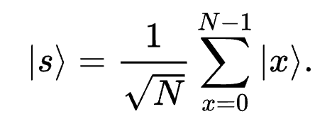
For a qubit and 2 states: 1/√2 |0⟩ + 1/√2 |1⟩

|ω⟩ and |s⟩ are not quite perpendicular because |ω⟩ occurs in the superposition with amplitude 1/√N

|s’⟩ = |s⟩ - |ω⟩ is perpendicular to |ω⟩

UₛUω |s⟩ (Grover’s diffuser) = 2 |s⟩⟨s| − I

The sum of oracle plus reflection is called Grover's iteration. To obtain the results the iteration is repeated O(√N) times.

How to test it in IBM’s Quantum Computer

To test Grover’s circuit on IBMQ, register here and get a token.

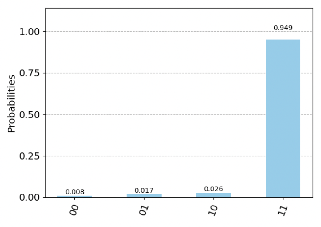
Here’s the code for 2 qubits:

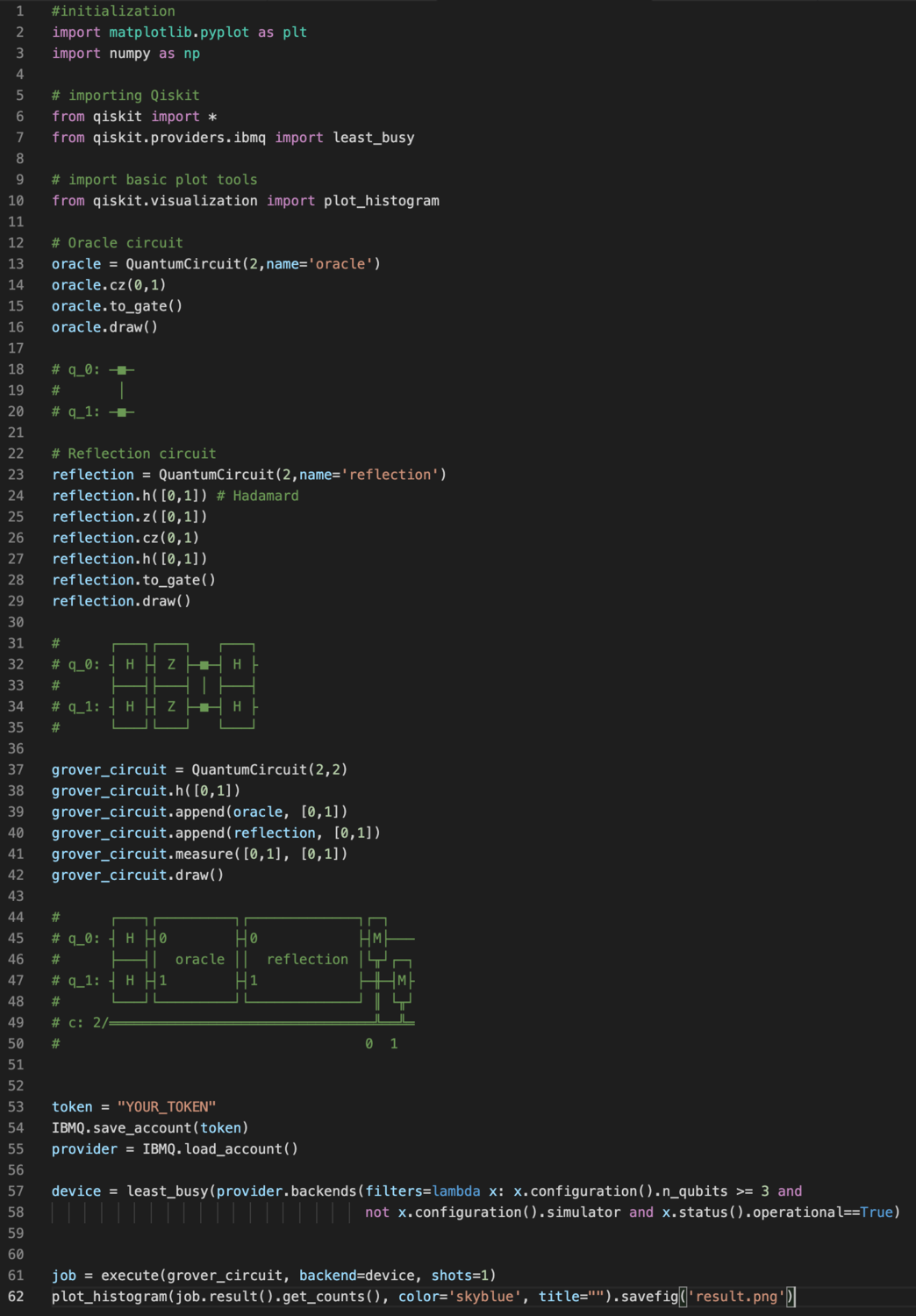
Probability of the winning state is 0.949